
Elevation Profile – The "Coastline Paradoxon’s" trap
Back to the main help page
The profile and derived values thereof
Let us assume that you upload a KML or GPX file with your last mountain hike in the map viewer. This KML or GPX file will be a line or a polygon consisting of multiple connected points containing values like the GPS position, the altitude, the time when created, etc. Our system allows you to automatically create an elevation profile provided by a backend service. Depending on the number of points, the profile will be more or less accurately resembling the «true» landscape’s features.

A number of different parameters is derived from this profile and the underlying coordinates:
- Highest Point
- Lowest Point
- Total Ascent
- Total Descent
- Total Distance
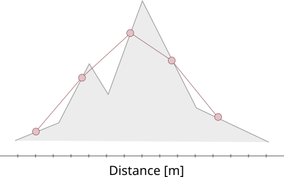
The highest and lowest points are trivial, being the max and min value of all altitudes.
For the total ascent (and likewise descent) we sum all positive (and likewise negative for descent) height differences between the adjoining points.
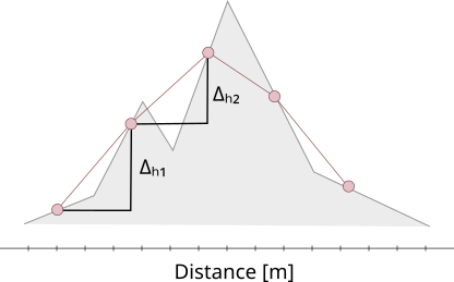
Even on this very simple sketch we can observe that the value for the total ascent will depend on the density of points, with the coarse distribution above we miss the little ditch on the left side, i.e. the total ascent would be higher than just Δh1 + Δh2.
The old viewer used a relatively coarse distribution of points along the track with point distances of ~100-200m. In certain cases, this caused problem, as important landscape features were missed (for example in the graph above, the highest point would not be accurately measured). With the launch of the new viewer, we wanted to improve that and increased the point density allowed. Now, every single point is considered (GPX track points have a mean distance of a few meters, depending on the device).

The "Coastline Paradox"
Does this mean that the more points your track has, the better result you will have? Unfortunately, this is not the case. Imagine that the point density is so big and thus the altitude values so accurate, that even walking over a rock would add ~50cm ascent on your path. This would result in a very steep ascent, even if the path is mainly horizontal.
This problem is also known as ‹Coastline Paradox› which is the counter-intuitive observation that «the coastline of a landmass does not have a well-defined length» (https://en.wikipedia.org/wiki/Coastline_paradox ).
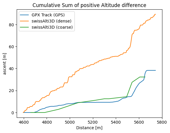
Let’s go back to a real-life example of a GPX track and analyse the height difference between the adjacent points:
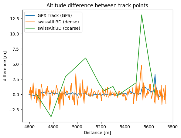
We observe that the difference in altitude between adjacent points is small for a dense point distribution compared to a coarse distribution. However, by summing up all the altitudinal differences we contrast becomes rather apparent.
Data accuracy
The underlying altitude data has a resolution of 2m and a vertical accuracy of less than 1m (below 2000m) / less than 5m (above 2000m). GPS points have a horizontal and vertical accuracy of ~5m (depending on the device, surrounding objects and landscape location). If we consider all these accuracy values, it becomes clear that small hight differences between close (i.e. a few meters) are within error margins and should not be considered.
The worst possible case would be a horizontal traverse along a steep slope: even a perfectly flat way would lead to a large total ascent if accurate altitude values and differences are derived from relatively inaccurate GPS locations.
The following picture illustrates the situation where the track follows a virtually horizontal path along a stone, but the track is slightly off the path

The profile is from the straight line more or less perpendicular to the track. For the point shown, if the track point was only registered 0.8m more to the right, the height would already be 2m lower.
Possible solution
Sia il vecchio che il nuovo visualizzatore di mappe servono per un'ampia gamma di applicazioni e non sono ottimizzati principalmente per l'elaborazione di percorsi GPS. Il calcolo dei valori derivati da un profilo, come descritto sopra, è quindi finora abbastanza semplice.
GPX Tracks
As GPS tracks are mostly transformed in GPX files, we will be focussing on them where 2 solutions are put in front of us:
- To simplify the response data
This can be done by only considering altitude differences larger than a certain threshold (like 1m.) - To simplify the input track
By applying the commonly used Douglas-Peucker algorithm (https://de.wikipedia.org/wiki/Douglas-Peucker-Algorithmus ) to reduce the number of points in the track by a factor of around 50-100 (for example, a track of 25'000 points would be
In a first step, we decided to apply the latter solution where the results would manifest in a coarse point distribution similar to the green line in the above graphics. The resulting altitude difference should be more plausible for GPX tracks and should serve better to observe the altimetry of your typical hiking tracks. However, we cannot avoid that this simplification leads to undesired results in very special cases that will be taking care internally with the time given.